Network Routing Algorithms#
These python scripts demonstrate two fundamental network routing algorithms: Bellman-Ford and Dijkstra. Both algorithms are used to find the shortest path in a network of routers, but they operate differently and have distinct use cases. Below are the implementations and explanations for each algorithm.
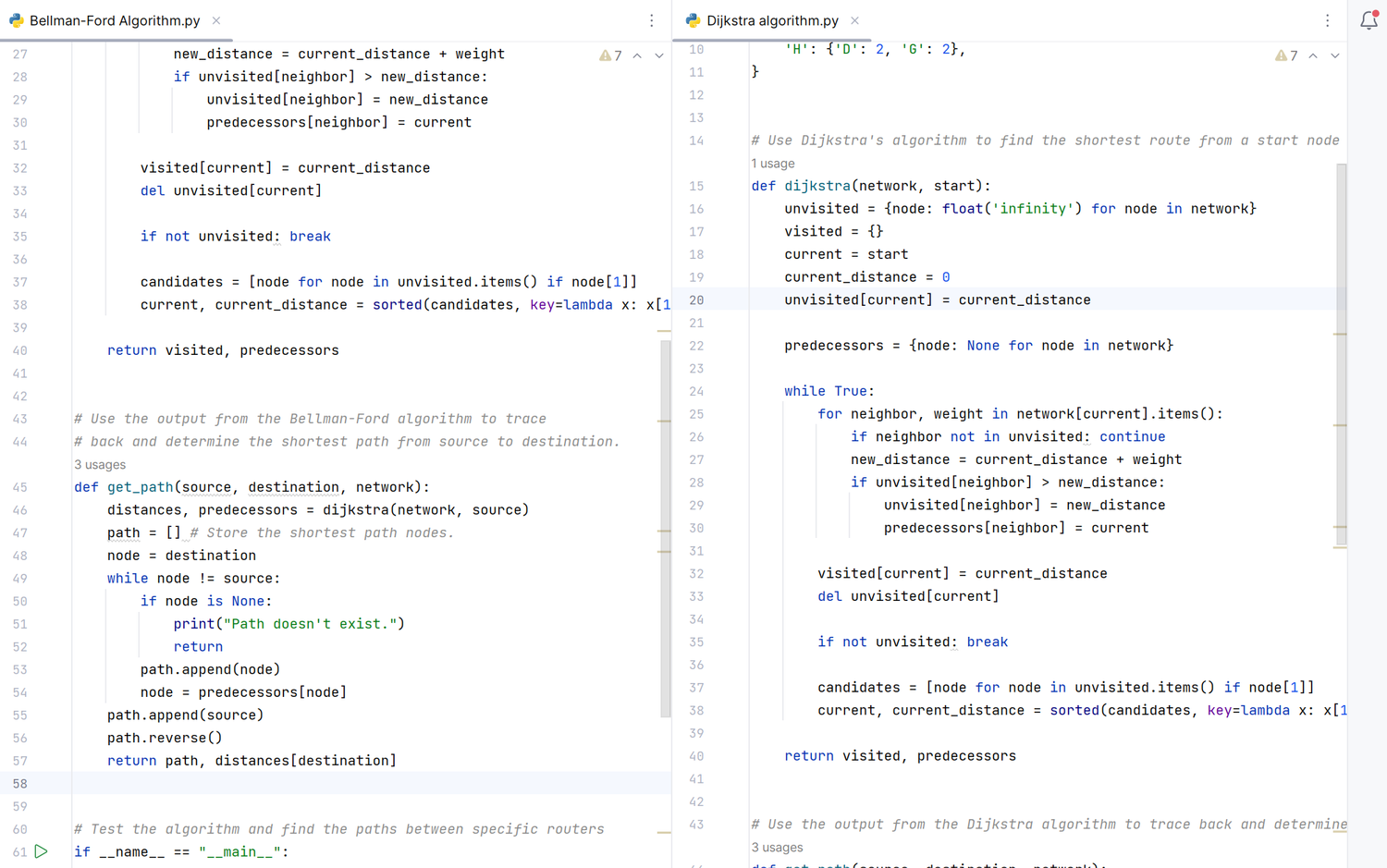
You can view the program code here:
Complexity, Advantages, and Disadvantages#
Bellman-Ford Algorithm#
Time Complexity:
The time complexity of the Bellman-Ford algorithm is \(O(V \cdot E)\), where \(V\) is the number of vertices and \(E\) is the number of edges.
Space Complexity:
The space complexity is \(O(V)\) for storing distances and predecessors.
Advantages:
Handles Negative Weights: Bellman-Ford can handle graphs with negative weight edges.
Detects Negative Weight Cycles: It can detect if there is a negative weight cycle in the graph, which Dijkstra’s algorithm cannot.
Disadvantages:
Slower than Dijkstra: Bellman-Ford is generally slower compared to Dijkstra’s algorithm for graphs without negative weights.
Inefficiency with Large Graphs: The algorithm can be inefficient for very large graphs due to its higher time complexity.
Dijkstra’s Algorithm#
Time Complexity:
Using a simple array: \(O(V^2)\)
Using a priority queue (e.g., binary heap): \(O((V + E) \log V)\)
Space Complexity:
The space complexity is \(O(V)\) for storing distances, predecessors, and the priority queue.
Advantages:
Efficiency: Dijkstra’s algorithm is faster and more efficient for graphs with non-negative weights.
Suitable for Dense Graphs: When implemented with a priority queue, Dijkstra’s algorithm performs well even for dense graphs.
Disadvantages:
Cannot Handle Negative Weights: Dijkstra’s algorithm cannot handle negative weight edges, as it may produce incorrect results.
No Cycle Detection: It does not detect negative weight cycles in the graph.